Marketing Mix Modeling: Why Experiments Must Anchor MMM

Adding experiments to a marketing mix model (MMM) is becoming table stakes. But simply passing experimental results into an MMM does not guarantee that the model will learn from them.

A model can fit historical sales extremely well, incorporate experiment results as a prior, and still produce the wrong answer about which channels drove incremental sales. For teams using MMM to guide budget decisions, that distinction matters.

The goal is not just an experiment-calibrated model. It is an experiment-anchored model: one whose final channel estimates remain consistent with the strongest causal evidence available.

Predictive fit is not causal fit

Marketing data is full of plausible explanations. During a promotion, for example, a company may increase spend across search, social, and video at the same time that underlying demand rises. A model must separate the sales generated by media from the sales that would have happened anyway.

Several channel mixes can explain the same total. One model might attribute $1 million to search and $3 million to social. Another might reverse those contributions. Both can reproduce the observed sales total, even though they imply very different budget decisions.

This is the difference between predictive and causal fit:

• Predictive fit asks whether the model can reproduce observed sales.
• Causal fit asks whether the model’s channel-level estimates agree with experimental evidence, accounting for uncertainty.

A credible causal marketing mix modeling approach needs both. Predictive accuracy helps the model explain the business. Experimental agreement helps establish whether its explanation is actually believable.

Experiments should anchor response curves

Experiments are most useful when they shape the model’s final response curves, not just its starting assumptions.

A common workflow is to use experiments to inform a prior, then update it with historical data. That can be directionally helpful, but it does not guarantee that the fitted model will remain consistent with the experiment. If historical sales exert enough influence, the posterior estimate can drift away from the measured result.

An experiment-anchored approach makes agreement with experiments an explicit objective for fitting. Haus’s posterior matching process checks the fitted response curves against experiments at the spend levels where those tests were run. When the estimates conflict with the evidence, the model updates and refits.

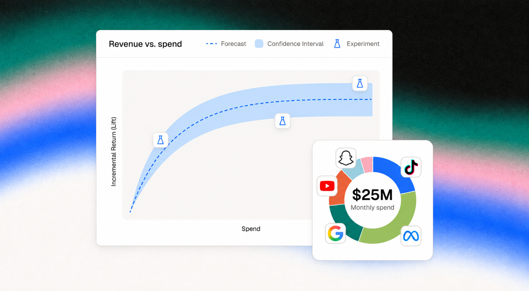
That spend-level context is important. A test at $20,000 and a test at $60,000 do more than provide two average ROI estimates. Together, they can reveal the shape of the response curve: how incremental sales change as spend increases and where diminishing returns begin. Collapsing both results into a single blended number throws away information budget planners need.

Uncertainty matters, too. The model should not be forced through every experiment’s point estimate as if each result were perfectly known. More precise experiments should carry more weight, while noisier measurements should widen the range of plausible response curves.

Timing changes what an experiment means

The same channel can produce different incremental returns in different periods. A test during a quiet month may produce a different result than a test during a major promotion, even at a similar spend level.

That does not mean one result is right and the other is stale. It means effectiveness may vary over time.

Time-varying return curves help put experiments from different periods on a common timing basis. This separates the effect of spending more from the effect of advertising when customers are more responsive.

In the Haus’ experiment-anchoring report’s simulation, a $35,000 test measured $32,000 in incremental sales, or 0.91 incremental return on ad spend (iROAS). The model estimated that media effectiveness during the test was 65% of its level in the reference period. On a common timing basis, the test implied approximately $49,000 in incremental sales, or 1.40 iROAS.

The 1.40 figure does not rewrite what the experiment measured. It makes the evidence comparable with tests conducted under different demand conditions. A quiet-period test can inform peak-season planning without assuming that effectiveness is constant all year. A peak-season test can inform ordinary periods without treating unusually favorable conditions as the norm.

Validate the model against experiments it has not seen

A model can agree with the experiments used during fitting and still fail to generalize. That is why causal marketing mix modeling needs a validation design that withholds experiments from the model.

In the report’s simulated business, the evaluation used three channels, nine experiments, and 520 days of sales history. Each experiment was left out in turn, and the model’s predicted lift was compared with the measured lift.

We found that adding experiments slightly worsened historical sales fit in this simulation, while substantially improving prediction on experiments the model had not seen. Adding timing improved both measures. The result highlights an important modeling tradeoff: A small sacrifice in fit to the total can be worthwhile if it produces a more credible estimate of what each channel caused.

Withholding a few weeks of sales is still a useful predictive check. But it does not answer the causal question. To test whether the model can anticipate the effect of deliberately changing spend, withhold an experiment.

Better causal estimates improve budget decisions

Response curves ultimately determine how much budget each channel receives. If a curve is wrong near the spend levels under consideration, the model misstates the return on the next dollar — and the budget inherits that error.

Timing adds another dimension. It can inform not only how much to spend, but when each channel is likely to work hardest.

In a separate constructed planning illustration from the report, three channels shared a $25 million quarterly budget under the same constraints. Compared with a plan based on sales history alone, the experiment-informed plan generated about $2.3 million more incremental sales, a 3% gain. Accounting for experiment timing increased the gain to about $3.8 million, or 5%.

These figures are illustrative rather than a forecast for any particular business. The broader point is practical: better causal estimates create the conditions for better allocation decisions.

The standard for an experiment-anchored MMM

Before trusting an MMM to direct the next dollar, ask four questions:

• Does the model fit historical sales?
• Do its channel effects agree with experiments, given uncertainty?
• Does it use experiments at the spend levels and timing conditions where they were run?
• Can it predict experiments that were withheld from fitting?

A model that answers only the first question may be predictive without being causal. A model that answers all four has a stronger basis for turning incrementality evidence into budget decisions.

Your experiments represent real operational work: spend was held back, tests were designed, and short-term performance may have been sacrificed to learn what actually works. Causal marketing mix modeling should make that work count—not merely by accepting experiments as inputs, but by allowing them to anchor what the model learns.

Read Haus’ full Causal MMM Experiment Anchoring Report

Haus Causal MMM is built to connect experimental evidence, time-varying effectiveness, and budget planning in one modeling workflow. Learn more about Haus Causal MMM.